Lab 2

Introduction

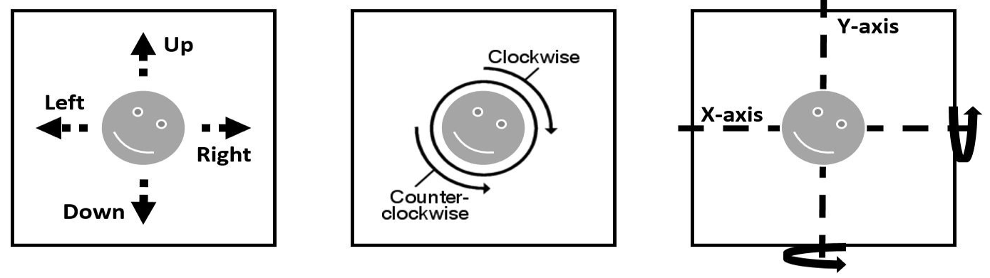
After great success with your previous client, OptsRus has a second client: a virtual reality headset startup. The startup is co-founded by a group of hardware geeks: those who like to design electrical circuits and integrate sensors. The VR headset prototype hardware is almost ready but lacks a high performance software image rendering engine. The hardware engineers have already wrote functionally correct code in C, but needs your help to supercharge the software performance and efficiency. The rendering engine’s input is a preprocessed time-series data set representing a list of object manipulation actions. Each action is consecutively applied over a 2D object in a bitmap image such that the object appears moving in reference to the viewer. In order to generate smooth and realistic visual animations, sensor data points are oversampled at 1500Hz or 25x normal screen refresh rate (60 frames/s). The image below shows all of the possible object manipulation action. Your goal is to process all of the basic object manipulation actions and output rendered images for the display at 60 frames/s.

Implementation Overview

Fundamentally, the rendering engine you are asked to optimize is very simple in design. This section will briefly describe all important parts you need to know for this lab. A well-documented trivial reference implementation is provided to help you get started.

Input Files

There are two files used as input. The first one is a standard 24-bit bitmap image file with a square dimension. The second one is a list of processed sensor values stored inside a csv (comma separated value) file. For the bitmap image file, white pixels (RGB=255,255,255) is considered as the background and non-white pixels are considered as part of an object. You can generate your own image files using Microsoft Paint in Windows or GIMP on Linux. After drawing your own square image, export the bitmap to 24-bit bitmap format. If you are using GIMP, make sure under the compatibility options, check "Do not write color space information" option. Then under advanced options, select "R8 G8 B8" under 24 bits. We packaged the a very tiny 10 x 10 pixel bitmap image named object_2D.bmp in the lab assignment package which helps you get started. The list of processed sensor values can be viewed as a list of key value pairs. The key represents a basic object manipulation action and the value is the magnitude of the specified action. An example sensor value input file is shown below:

W,6     // shift object up by 6 pixels
A,5     // shift object left by 5 pixels
S,4     // shift object down by 4 pixels
D,3     // shift object right by 3 pixels
CW,2    // rotate entire image clockwise by 180 degrees
CCW,1   // rotate entire image counter clockwise by 90 degrees
MX,1    // mirror entire image along the X-axis in the middle
MY,0    // mirror entire image along the Y-axis in the middle

Data Structures

Frame Buffer and Dimension

The input bitmap image has already been parsed for you. The image pixel data is stored into the following data structure below:

unsigned char *frame_buffer;    // [R1][G1][B1][R2][G2][B2]...
unsigned int width, height;     // dimension in number of pixels

Sensor Values

The processed sensor values input file has also been parsed for you and stored inside a key value pair array. The array has enough storage for more than 10,000 key value pairs. As mentioned earlier, the key represents the basic object manipulation action and value represents the magnitude. It is stored in the following data structure below:

// KV Data Structure Definition
struct kv {
  char *key;
  int value;
};
// KV Data Structure Array
struct kv sensor_values[10240];

Key Function and Definitions

In this lab, you are only allowed to modify a single file (implementation.c). Inside this file, there are two important function which you should take extra precaution.

implementation driver()

This method is the main entry point to your code. All of the available data is passed to your implementation via this function. You should not modify the prototype of this function. Currently, a naive but working solution of the lab inside implementation_driver() is provided to help you get started. However, you are free to modify the implementation of this function as well modify and delete anything else in this file. Please make sure the implementation_driver() function is always reachable from main.

The prototype of the function is the following:

void implementation_driver(
   struct kv *sensor_values, int sensor_values_count,
   unsigned char *frame_buffer,
   unsigned int width, unsigned int height,
   bool grading_mode
);

verifyFrame()

You must call this function for each frame you are required to output. Before you call this function, please make sure the you pass in valid data of the correct type. Failing to do this step will generate error in the program thus failing implementation verification check.

The prototype of the function is the following:

void verifyFrame(unsigned char *frame_buffer,
                 unsigned int width, unsigned int height,
                 bool grading_mode);

Performance Measurement of the Tool

perf

To gain insight into the cache behavior of your implementation, you can use the perf infrastructure to access the hardware performance counters of the processor. For example, to output the first-level cache misses generated by your program foo you would execute:

perf stat -e L1-dcache-load-misses foo

You can view a listing of all performance counters that you can monitor by running:

perf list

Note that you can monitor multiple counters at once by using multiple -e options in one command line. perf has many other features that you can learn more about by browsing:

perf --help

For example, you can consider monitoring TLB misses or other more advanced events. A small write-up on perf is available here: http://www.pixelbeat.org/programming/profiling/

Unfortunately there is not a lot of documentation on perf yet as it is so new, but the "help" information is clear.

Gprof & GCov

If you have successfully completed lab1, you should be familiar with these two tools. They can be very useful in pin-pointing the bottleneck of your program running locally.

Note: To configure these tools to use within your project, you will need to provide additional meson commandline options while generating build directory.

Setup

Ensure you're in the ece454 directory within VSCode. Make sure you have the latest skeleton code from us by running: git pull upstream main.

This may create a merge, which you should be able to do cleanly. If you don't know how to do this read Pro Git. Be sure to read chapter 3.1 and 3.2 fully. This is how software developers coordinate and work together in large projects. For this course, you should always merge to maintain proper history between yourself and the provided repository. You should never rebase in this course, and in general you should never rebase unless you have a good reason to. It will be important to keep your code up-to-date during this lab as the test cases may change with your help.

The ONLY files you will be modifying and handing in is implementation.c. You are prohibited to modify other files. You can finally run: cd lab2 to begin the lab.

Compilation

First, make sure you're in the lab2 directory if you're not already. After, run the following commands:

meson setup build
meson compile -C build

Whenever you make changes, you can run the compile command again. You should only need to run setup once. If you do need to try other flags, it's best to remove the build directory (rm -rf build) and run meson setup build again.

The executable to run will be build/lab2.

Coding Rules

The coding rules are very simple. You may write any code you want, as long as it satisfies the following:

• You submission have only the modified implementation.c file and not any other file. You are not allowed to modify the meson.build file, and as a result, you will not be able to bypass this limitation.
• You must not interfere or attempt to alter the time measurement mechanism.
• Your submitted code does not print additional information to stdout or stderr.

Evaluation

The lab is evaluated when the grading mode is turned on. The grading mode previously mentioned in many sections is controlled via an additional flag -g option flag via command line (see example terminal output below). The evaluation turns on instrumentation code which measures the total clock cycle used by the implementation_driver() function. When you evaluate your implementation using the command below, you should receive similar output.

build/lab2 -g -f sensor_values.csv -i object_2D.bmp
Loading input sensor input from file: sensor_values.csv
Loading initial 2D object bmp image from file: object_2D.bmp
************************************************************************************
Performance Results:
   Number of cpu cycles consumed by the reference implementation: 124374
   Number of cpu cycles consumed by your implementation: 125073
   Optimization Speedup Ratio (nearest integer): 1
************************************************************************************

Marking Scheme

Note: for 2024 Fall, this is subject to change.

Note: This course also allow you to practice optimizing for your time and grades. Don’t be too stressed over the fact that there will be people who are better at optimizing the program than you are. However, you should be worried if you cannot meet the minimal and acceptable performance targets.

Non-Competitive Portion Level - 80%

The non-competitive portion should be fairly easy for everyone who puts in the good amount of effort. If you can achieve this level of performance improvement, the TA will assign marks to you for this portion. The speedup threshold will be the average mark of all submissions in the first week from last year (100x speedup). TA reserves the right to decrease the performance threshold to obtain the 80% mark if there are students struggling even after putting in serious amount of efforts (determined by the TA).

Competitive Portion - 20%

This lab is designed to have very high potential for performance optimization. One can trivially achieve at least 50x performance speedup compared to the reference solution. Once you submit your work using the usual submitece command, your submission will be placed onto a queue for auto-grading.

The competitive portion’s marks (20% of total marks) will be assigned based on your performance tier, to be determined.

Note: The input we used to evaluate your solution is purposely not provided. It is to prevent students from hard coding optimized solution to the input. However, you should expect the image size to be large (somewhere around 10,000 x 10,000) with a long list of commands.

The competitive portion of the mark should be available via a web portal within maximum of 24hrs. In most cases, your updated score should be reflected on the web portal automatically within a very short period of time. The marks you see on the web portal is only for reference and mostly accurate. It would be adjusted if cheating behavior is observed. The web portal’s URL is the following: https://compeng.gg/ece454/ (may have initial problems).

Assignment Assumptions

In the auto-grader, you can/should assume the following points when writing your algorithm:

1. Object will always be visible and never shifted off the image frame.
2. Don’t need to output incomplete frames (image frame composing of less than 25 object manipulating actions)
3. Solution will only need to handle square image with size up to 10,000 pixels in width and height.
4. Solution will only need to perform maximum of 10,000 sensor value inputs.
5. Your solution is evaluated multiple times before an average speedup is taken. You shall not cache the final output results from prior runs to gain advantage. Doing so will be considered cheating.
6. As long as your code compiles with modifications only in implementation.c file and have not attempted to cheat, your solution is most likely valid. If in doubt, as the TA via e-mail or on Discord.
7. Your solution will be tested on a single dedicated machine. The dedicated machine (for now) is a Raspberry Pi 4. The speedup of your optimized program can viewed through the web portal. The web portal is designed with a delay to show the speedup scores to prevent students from submitting too frequently. We highly recommend you to use ug lab machine to test for correctness and gauge a relative performance against your previous solutions. However, your final grades will be assigned via performance measurement generated on the dedicated machine (available on the web portal).

Submission

Simply push your code using git push origin main (or simply git push) to submit it. You need to create your own commits to push, you can use as many as you'd like. You'll need to use the git add and git commit commands. You may push as many commits as you want, your latest commit that modifies the lab files counts as your submission. For submission time we will only look at the timestamp on our server. We will never use your commit times (or file access times) as proof of submission, only when you push your code to GitHub.